
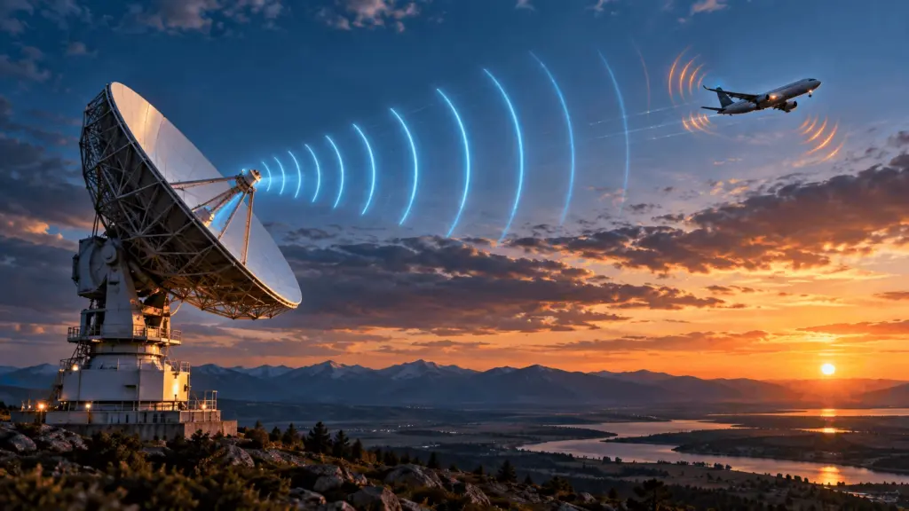
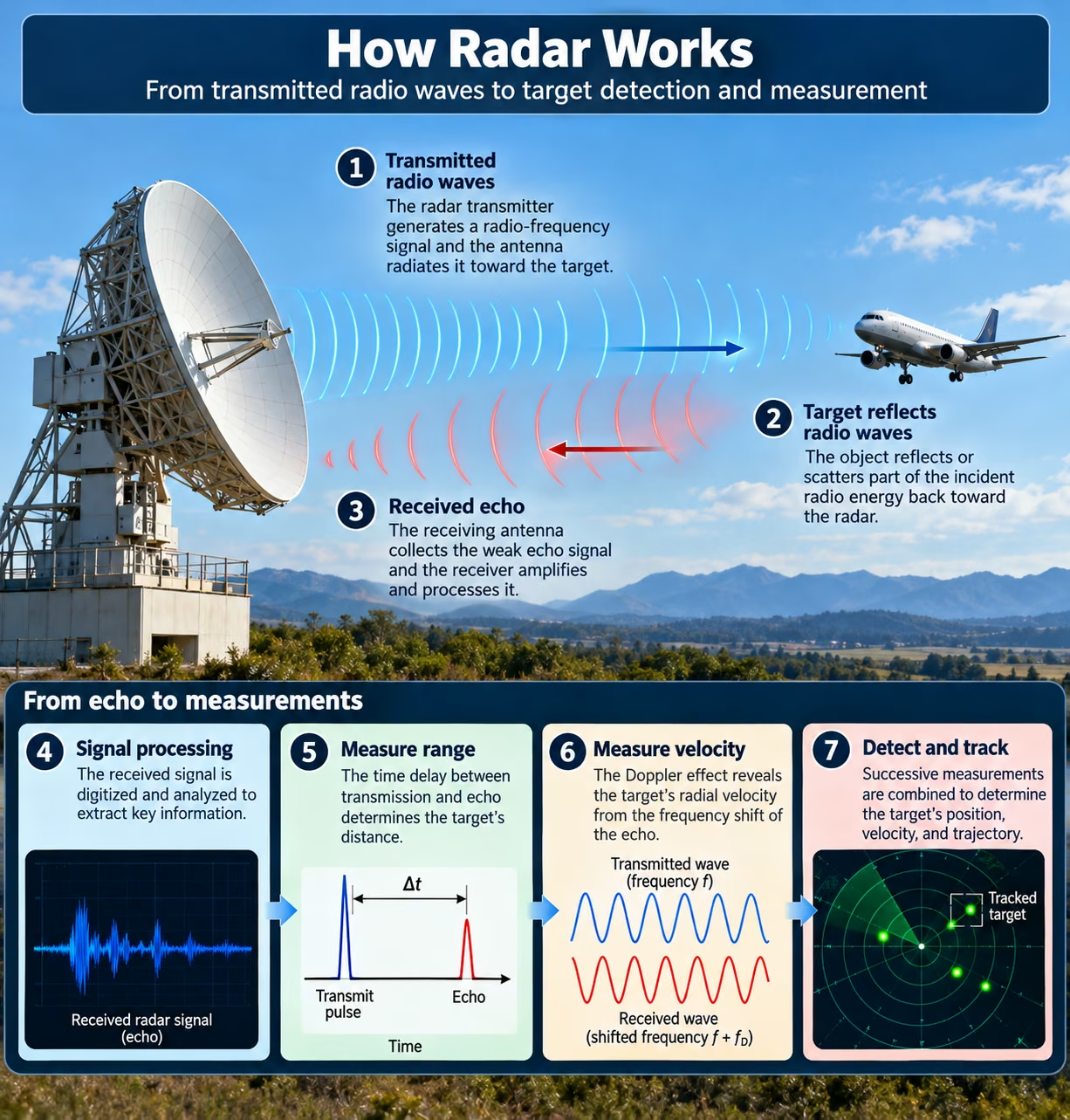
Radar allows us to detect an aircraft flying through clouds, measure the speed of a moving vehicle, monitor rainfall inside a thunderstorm, and help cars recognize obstacles in darkness. Although these applications seem different, they rely on the same fundamental physics: electromagnetic waves interact with objects, and the returning signals reveal information about their position and motion.
Radar stands for Radio Detection and Ranging. It is an active sensing technology that transmits radio-frequency electromagnetic energy and analyzes the signals reflected or scattered back from objects. Depending on the radar design, these measurements can reveal an object’s distance, direction, radial velocity, and other characteristics.
Three physical principles explain most radar measurements:
- Radio-wave propagation: Electromagnetic waves travel at nearly the speed of light in air.
- Time of flight: The time required for a signal to reach an object and return reveals its distance.
- Doppler effect: Motion toward or away from the radar changes the frequency or phase progression of the received signal, allowing radial velocity to be estimated.
Unlike optical cameras, radar does not need sunlight or visible illumination. Many radar frequencies can also operate through clouds, fog, and some precipitation. However, heavy rain, atmospheric absorption, interference, terrain, and the radar’s operating frequency can limit its performance.
This guide explains how radar works, why it uses radio waves, how engineers calculate distance and speed, and how technologies such as pulse-Doppler radar, FMCW radar, phased arrays, and digital signal processing turn weak electromagnetic echoes into useful measurements. [1][2]
1. What Is Radar and How Does It Work?
Radar is a remote-sensing system that measures objects without physical contact. A conventional radar emits electromagnetic energy, receives part of the energy scattered by objects, and processes the return. The radar can estimate an object’s position and movement even when it cannot be seen by the human eye. Whether a system monitors aircraft, vehicles, ships, or rainfall, its underlying task is to extract reliable information from radio signals that may be extremely weak compared with the original transmission.
1.1. What Does Radar Stand For?
The acronym RADAR comes from Radio Detection and Ranging. Detection means deciding whether a target is present, while ranging means estimating the distance between the radar and that target. Modern radar systems can also measure radial velocity, estimate direction, and track objects over time.
Several terms are important:
- Radar signal: The transmitted or received electromagnetic waveform.
- Radar echo: Energy scattered from an object and received by the radar.
- Target detection: The identification of a return considered likely to represent an object.
- Radar range: The distance measured along the radar’s line of sight.
- Target tracking: The process of connecting observations to estimate an object’s continuing motion.
Radar differs from other sensing technologies primarily in the waves it uses.
| Technology | Sensing method | Common uses |
|---|---|---|
| Radar | Radio-frequency electromagnetic waves | Vehicles, aircraft, weather, surveillance |
| Lidar | Laser light | Mapping, robotics, autonomous sensing |
| Sonar | Acoustic waves | Underwater detection, depth measurement |
| Optical camera | Visible light | Photography, visual recognition |
The development of practical radar accelerated during the 1930s. Scottish physicist Robert Watson-Watt played an important role in Britain’s early radar development, although the technology resulted from contributions by many scientists and engineers internationally.
1.2. How Does Radar Detect an Object?
A radar detects an object by transmitting a signal and analyzing energy that returns after interacting with the environment. Because objects reflect and scatter radio waves differently, the radar must distinguish useful echoes from background clutter, interference, and receiver noise.
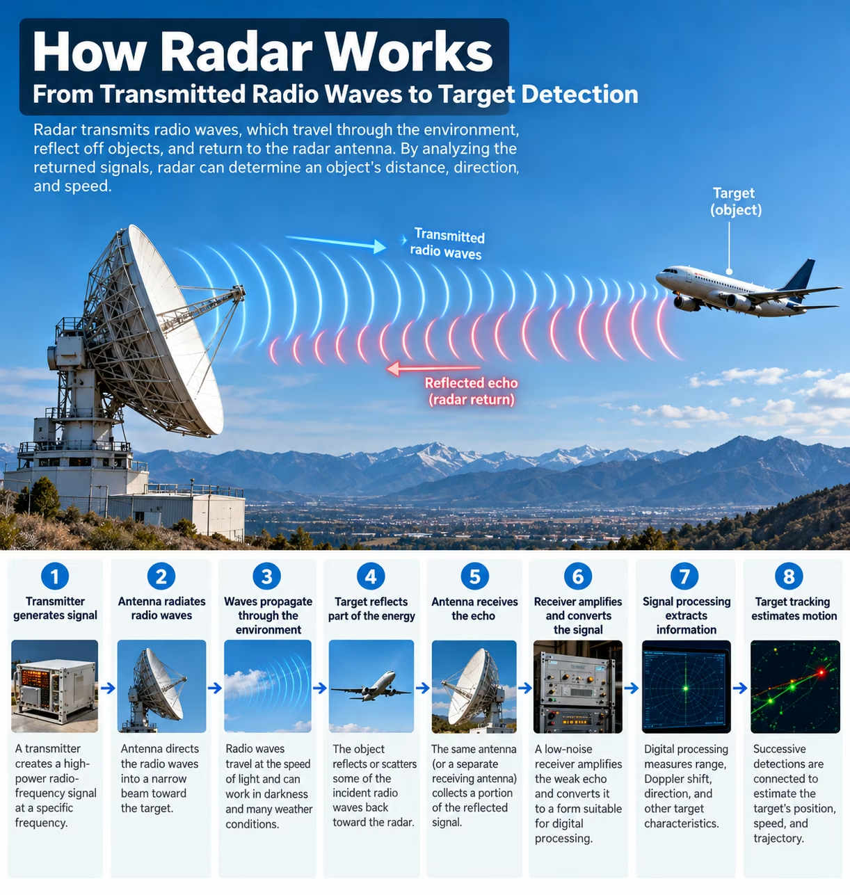
The detection process involves eight steps:
- The transmitter generates a radio-frequency waveform.
- The antenna directs electromagnetic energy into space.
- The radio wave propagates through the environment.
- An object scatters or reflects some incident energy.
- The receiving antenna collects a small portion of the return.
- The receiver amplifies, converts, and digitizes the signal.
- Digital processing estimates target measurements and identifies significant returns.
- Tracking algorithms associate detections across successive observations.
Not every transmitted signal produces a detectable echo. Successful detection depends on the target’s scattering properties, propagation conditions, system sensitivity, and the processing methods used. [1]
1.3. What Information Can Radar Measure?
Radar can provide several types of measurements, although their availability depends on its hardware and waveform. A basic pulsed radar might measure distance and horizontal direction, while a modern coherent radar with multiple antennas can estimate range, radial velocity, azimuth, and elevation.
| Measurement | Meaning | Typical measurement method |
|---|---|---|
| Range | Distance to the object | Echo delay or waveform modulation |
| Radial velocity | Motion toward or away from radar | Doppler shift |
| Azimuth | Horizontal bearing | Antenna pointing or array processing |
| Elevation | Vertical angular direction | Vertical beam or antenna array |
| Reflectivity or echo strength | Strength of returned energy | Received signal power |
| Target classification | Probable object category | Features and pattern analysis |
Importantly, a radar’s Doppler measurement does not automatically reveal an object’s complete three-dimensional velocity. It normally measures only the component along the radar’s line of sight. Determining full motion may require observations from different viewing angles, multiple sensors, or tracking over time.
2. Why Does Radar Use Radio Waves?
Radio waves are particularly useful for detecting objects at a distance because they can travel through the atmosphere, be directed by antennas, and carry measurable timing, amplitude, frequency, phase, and polarization information. Their behavior is governed by electromagnetic physics. Depending on frequency, radar waves can travel over substantial distances, interact with precipitation, penetrate certain materials, or provide fine measurement resolution. Engineers select radar frequencies by balancing these advantages against practical constraints such as antenna size, atmospheric absorption, available bandwidth, and regulatory spectrum allocations.
2.1. What Are Radio Waves?
Radio waves are electromagnetic waves consisting of oscillating electric and magnetic fields. These fields propagate through space and transport electromagnetic energy. Radio waves belong to the same electromagnetic spectrum as infrared radiation, visible light, ultraviolet radiation, X-rays, and gamma rays, but generally have lower frequencies and longer wavelengths.
James Clerk Maxwell established the theoretical foundation of electromagnetic-wave propagation through his equations of electromagnetism. Heinrich Hertz later demonstrated electromagnetic waves experimentally.
Radar commonly operates in the microwave portion of the radio spectrum, extending from roughly 300 MHz to 300 GHz under a widely used definition. Microwave frequencies are useful because relatively compact antennas can form directional beams, and their signals interact with objects at scales relevant to radar detection.
2.2. How Are Frequency and Wavelength Related?
Frequency describes how many wave cycles occur each second, measured in hertz (Hz). Wavelength is the physical distance between corresponding points on consecutive cycles, measured in meters.
In a vacuum, electromagnetic waves travel at the speed of light:
The fundamental relationship is:
Therefore:
Here, f is frequency and λ is wavelength.
A 3 GHz radio signal has a wavelength of approximately 10 centimeters, while a 30 GHz signal has a wavelength of approximately 1 centimeter. Increasing the frequency by a factor of ten reduces the wavelength by the same factor.
Inside materials, the wave’s phase velocity and wavelength depend on the material’s electromagnetic properties. For radar calculations in air, approximately 3×10⁸ m/s is ordinarily a useful approximation.
2.3. Which Radio Frequencies Are Used in Radar?
Radar systems operate across multiple frequency bands because no single frequency offers optimal performance for every application. Lower frequencies generally offer different propagation and penetration characteristics, whereas shorter wavelengths can support compact antennas and high angular resolution for a fixed antenna aperture.
The following frequency ranges use common IEEE radar-band terminology. Actual equipment bands and national allocations may differ.
| Radar band | Approximate frequency | Typical applications |
|---|---|---|
| L-band | 1–2 GHz | Surveillance, long-range sensing |
| S-band | 2–4 GHz | Weather radar, air surveillance |
| C-band | 4–8 GHz | Weather radar, satellite sensing |
| X-band | 8–12 GHz | Marine radar, imaging, tracking |
| Ku-band | 12–18 GHz | Specialized sensing and tracking |
| K-band | 18–27 GHz | Short-range and specialized radar |
| Ka-band | 27–40 GHz | High-frequency radar applications |
| Millimeter-wave region | Approximately 30–300 GHz | Automotive, industrial, high-resolution sensing |
Modern automotive radar commonly operates around 77 GHz, which lies within the millimeter-wave region.
Frequency alone does not determine range resolution. For a typical bandwidth-limited radar waveform, range resolution depends primarily on transmitted signal bandwidth, while angular resolution depends on factors including wavelength, aperture size, and array processing.
2.4. How Do Radio Waves Travel Through the Environment?
Radar propagation is influenced by the atmosphere, terrain, obstacles, and electromagnetic reflections. Under many operating conditions, radar beams travel approximately along straight paths, but atmospheric refraction can bend them, and Earth’s curvature may restrict the direct visibility of distant low-altitude targets.
Several propagation effects matter:
- Radar horizon: The approximate geometric or refracted line-of-sight limit for detecting targets near Earth’s surface.
- Free-space path loss: Reduction in power density as a wave spreads through space.
- Atmospheric attenuation: Energy loss caused by absorption and scattering, including effects from oxygen, water vapor, and precipitation.
- Multipath propagation: Reception of signals that traveled along different reflected paths.
- Radio-frequency interference: Unwanted electromagnetic energy from other transmitters or sources.
These effects are not equally severe at every frequency. Millimeter-wave radar can experience significant atmospheric absorption at particular frequencies, while lower-frequency systems often have different coverage and penetration advantages.
Radar may operate effectively through clouds and fog, but it should not be described as completely unaffected by weather. [1][3]
3. What Are the Main Components of a Radar System?
A radar system combines radio-frequency electronics, antennas, receiving circuits, digital processing hardware, and tracking software. The transmitter produces the waveform, the antenna radiates and collects energy, and the receiver converts weak returning signals into usable electronic data. Modern radar processing then estimates target parameters, detects potential objects, and maintains their tracks. Although the implementation varies significantly between a weather radar installation and a compact automotive sensor, their functional building blocks are closely related.
3.1. Radar Transmitter: How Are Radio Signals Generated?
The radar transmitter produces the electromagnetic signal that will be radiated through the antenna. It usually includes a frequency source, modulation circuitry, and one or more power amplification stages. An RF oscillator establishes a frequency reference, while waveform-generation circuits control pulse timing, frequency modulation, or phase modulation.
Historically, high-power radar transmitters frequently used vacuum-tube devices such as magnetrons and klystrons. Modern systems also employ solid-state amplifiers, which can offer precise waveform control, modularity, and reliability.
Transmitters may generate short pulses, continuous signals, or frequency-swept waveforms. Increasing transmitted energy can improve the detection of weak echoes, but radar range depends on additional factors including antenna gain, target scattering, noise, and losses.
3.2. Radar Antenna: How Are Radio Waves Directed?
A radar antenna converts electrical signals into electromagnetic radiation and performs the reverse operation when receiving waves. Its design influences the direction, strength, and angular distribution of the radar beam.
Antenna gain describes the concentration of radiated power relative to a reference antenna. Directivity describes how strongly radiation is concentrated in particular directions, while beamwidth characterizes the angular width of a beam.
A narrow beam helps separate objects at different bearings. However, obtaining a narrow beam generally requires a larger electrical aperture.
Radar antennas also use polarization, commonly horizontal, vertical, or circular. The polarization of an echo depends on the transmitted wave and the scattering target. Weather radars can exploit polarization differences to obtain additional information about precipitation.
3.3. What Is a Phased Array Radar?
A phased array radar uses multiple antenna elements whose signals are combined with controlled phase relationships or more general complex weights. By changing these relationships, the system can steer its radar beam electronically without relying solely on mechanical antenna rotation.
This process is called beamforming. Constructive and destructive interference between signals from the elements creates a directional radiation pattern.
Two important architectures are passive electronically scanned arrays (PESA) and active electronically scanned arrays (AESA).
PESA systems generally distribute signals from a central high-power transmitter, while AESA systems use distributed transmit-and-receive electronics associated with antenna elements or groups.
Electronic steering can provide rapid scanning, flexible beam scheduling, and simultaneous or interleaved radar functions, although practical performance is limited by hardware, processing capacity, power, and beam-management requirements.
3.4. Radar Receiver: How Are Weak Echoes Detected?
The radar receiver must extract useful information from reflected signals that may be many orders of magnitude weaker than the transmitted waveform.
A common receiving chain begins with a low-noise amplifier (LNA), which increases the signal level while introducing as little additional noise as practical.
A mixer and local oscillator may convert the received RF signal to an intermediate frequency or directly to baseband. Filtering limits unwanted frequency components before an analog-to-digital converter (ADC) produces digital samples.
Many coherent receivers generate in-phase (I) and quadrature (Q) signal components. These preserve complex amplitude and phase information, enabling more complete Doppler and direction-sensitive processing.
Receiver performance is described using metrics such as noise figure, sensitivity, dynamic range, and linearity. A sensitive receiver is valuable, but a poorly managed noise floor or interference environment can still prevent reliable detection.
3.5. How Does Signal Processing Turn Echoes Into Measurements?
Raw receiver samples rarely provide useful target measurements without processing. Digital radar systems apply filtering, correlation, spectral analysis, detection algorithms, and tracking methods to estimate what objects are present.
The Fourier transform represents a signal in terms of its frequency components. Its computational implementation, the fast Fourier transform (FFT), is widely used in radar signal processing.
For example, a pulse-Doppler radar can compare the phase progression of repeated echoes to estimate velocity. An FMCW radar may perform a range FFT followed by a Doppler FFT to construct a two-dimensional representation of targets.
The signal processor must also distinguish meaningful peaks from thermal noise, interference, and clutter. Detected measurements are then passed to tracking algorithms that maintain estimates of object position and motion. [1][4]
4. How Does Radar Measure Distance Using Radio Waves?
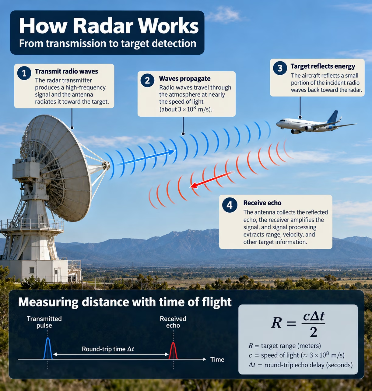
The simplest radar distance measurement is based on time. A radar transmits a pulse, records when it was sent, and determines when its echo returns. Because the radio wave travels from the radar to the target and back, the measured travel time corresponds to twice the target distance. Accurate ranging therefore requires a known propagation speed, reliable timing, and a way to associate a received echo with its transmitted waveform.
4.1. What Is Time of Flight in Radar?
Time of flight describes the travel time of an electromagnetic signal between two points. For conventional monostatic radar, the same site transmits and receives, so the measured echo delay represents a round trip.
If a target is 1,500 meters away, the signal travels approximately 3,000 meters in total. At 3×10⁸ meters per second, the round-trip time is approximately 10 microseconds.
In pulsed radar, a short transmission establishes a timing reference. The receiver then measures returning echoes at different delays.
Accurate time-of-flight measurement is particularly important when several objects are located at different distances within the same antenna beam.
4.2. How Is Radar Range Calculated?
The fundamental monostatic range equation is:
Where:
- R = target range in meters
- c = electromagnetic propagation speed in meters per second
- Δ t = measured round-trip delay in seconds
The division by two is essential because the signal travels to the target and then returns.
For a target located 15 kilometers away, the total propagation distance is approximately 30 kilometers. Dividing that distance by the signal’s propagation speed gives a round-trip delay of approximately 100 microseconds.
This equation assumes a known propagation speed and direct signal path. High-precision applications may need additional corrections for propagation and system delays.
4.3. Example: How Far Away Is a Target if Its Echo Returns After 20 Microseconds?
Suppose a radar transmits a pulse and receives a corresponding echo after 20 microseconds. We can calculate its target distance by converting the delay to seconds and using the round-trip range equation.
The target is approximately 3 kilometers from the radar, assuming a direct propagation path.
This example illustrates the scale of radar timing: just one microsecond of additional round-trip delay corresponds to approximately 150 meters of additional range.
4.4. What Is a Range Gate?
A range gate is a selected time interval in which the radar examines returning signals. Because echo delay corresponds to distance, selecting a particular delay interval effectively selects a particular range interval.
For example, a radar could analyze echoes expected from targets between 2 and 3 kilometers away while ignoring returns outside that window.
Modern digital radars frequently divide their observations into range bins, which are discrete intervals representing different distances.
Range gating can reduce unnecessary processing and help distinguish groups of targets at different ranges. However, it does not independently guarantee separation of targets that lie closer together than the radar’s effective range resolution.
4.5. What Is Range Resolution?
Range resolution is the radar’s ability to distinguish two targets at slightly different distances. It is different from range accuracy, which describes how closely an estimated distance agrees with the true distance.
For a simple uncompressed rectangular pulse of duration τ, the nominal range-resolution relationship is:
A pulse lasting 1 microsecond corresponds to approximately 150 meters of nominal range resolution.
For a suitable bandwidth-limited waveform with effective bandwidth B, a widely used approximation is:
This means that increasing waveform bandwidth can improve the ability to resolve closely spaced targets.
Resolution also depends on waveform design, processing, windowing, and the definition used to distinguish two returns. A radar may estimate the location of a single strong target more precisely than its nominal ability to resolve two nearby targets.
4.6. How Does Pulse Compression Improve Range Resolution?
Pulse compression allows a radar to transmit a relatively long, energetic pulse while achieving the range resolution associated with a much shorter effective pulse.
Instead of transmitting an unmodulated pulse, the radar introduces a controlled frequency or phase modulation pattern. A common waveform is a linear frequency-modulated chirp, whose instantaneous frequency changes approximately linearly during transmission.
On reception, matched filtering correlates the received signal with an expected waveform and concentrates its energy into a narrow response.
Consequently, the radar can benefit from substantial transmitted pulse energy without being restricted to the coarse range resolution of an equally long unmodulated pulse.
Pulse compression is used in many modern surveillance, imaging, and weather radar systems, although practical filtering introduces considerations such as sidelobes and processing losses. [1][4]
5. What Determines a Radar’s Maximum Detection Range?
A radar’s maximum detection range depends on how much transmitted energy reaches a target, how strongly the target scatters that energy back, and whether the receiver can distinguish the return from noise and interference. Greater transmitted power does not translate directly into a proportional increase in distance because radar echoes weaken rapidly as target range increases. Engineers use the radar range equation to understand this relationship and evaluate antenna gain, radar cross section, receiver sensitivity, operating wavelength, and propagation losses.
5.1. What Is the Radar Range Equation?
The radar range equation describes the relationship between transmitted power and the power received from a target. For an idealized monostatic radar, where transmission and reception occur at the same location, a commonly used equation is:
| Symbol | Meaning | Unit |
|---|---|---|
| Pr | Received power | Watts |
| Pt | Transmitted power | Watts |
| G | Antenna gain, assumed equal for transmission and reception | Dimensionless |
| λ | Radar wavelength | Meters |
| \sigma | Radar cross section | Square meters |
| R | Target distance | Meters |
| L | Combined system loss factor | Dimensionless, ≥ 1 |
The equation assumes free-space propagation, far-field conditions, a point-like target representation, and appropriate antenna alignment. It also uses linear power and gain values rather than decibel values.
It describes received signal power, not detection probability directly. To estimate detection range, the received power must be compared with the receiver’s noise characteristics and required detection performance. [1]
5.2. Why Does a Radar Echo Become Weaker With Distance?
Radar echoes weaken with distance because electromagnetic energy spreads as it travels outward, and the scattered energy spreads again as it returns. In the ideal monostatic point-target model, this produces an inverse fourth-power relationship:
If all other factors remain unchanged and the target distance doubles:
The received power becomes one-sixteenth of its original value, corresponding to approximately a 12 dB reduction.
This steep reduction explains why detecting a distant, weakly reflecting target is difficult. Atmospheric attenuation, interference, and other losses can further reduce performance beyond the ideal free-space prediction.
5.3. What Is Radar Cross Section?
Radar cross section (RCS) describes how strongly an object scatters electromagnetic energy in a specified direction under particular measurement conditions. It is expressed in square meters, but it is not simply the physical surface area of the object.
A target’s RCS depends on several factors, including its shape, material, orientation, size relative to wavelength, polarization, and observing frequency.
For example, a flat conducting surface may produce a strong return when oriented appropriately toward a radar, yet a much weaker return from another viewing angle.
Complex objects may contain multiple scattering points whose reflected fields reinforce or cancel one another.
Consequently, a physically large object can have a relatively small radar cross section in a particular direction, while a smaller object or specially shaped reflector can produce a strong return.
5.4. How Do Antenna Gain and Receiver Sensitivity Affect Detection Range?
Antenna gain improves radar performance by concentrating transmitted energy in useful directions and enhancing reception from those directions. In the simplified monostatic radar equation, antenna gain appears twice because the antenna influences both transmission and reception.
Receiver sensitivity determines how weak a signal can be while still satisfying a specified measurement or detection criterion.
The receiver’s noise floor depends on thermal noise, noise figure, receiver bandwidth, and processing characteristics. A simple thermal-noise relationship is:
Where k is Boltzmann’s constant, T is reference noise temperature, B is receiver noise bandwidth, and F is the linear noise factor, under the corresponding reference assumptions.
Detection generally becomes more reliable as signal-to-noise ratio (SNR) improves. However, the required SNR depends on target fluctuations, integration time, detector design, and acceptable false alarm probability.
5.5. Why Is Detection Range Different From Unambiguous Range?
Maximum detection range and maximum unambiguous range describe different limitations.
Maximum detection range refers to how far away a target can be detected under specified conditions. It is principally related to signal strength, noise, and detection criteria.
Maximum unambiguous range refers to the distance interval within which a conventional pulse radar can associate returning echoes with transmitted pulses without confusion.
For a simple pulse radar operating at pulse repetition frequency (PRF):
For example, at 1,000 pulses per second:
The nominal unambiguous range is 150 kilometers.
A radar might have adequate sensitivity to detect a target beyond this distance, yet incorrectly assign its echo to a later transmitted pulse. Advanced radar systems employ techniques such as varying PRFs, coded pulses, and ambiguity-resolution processing to address this problem. [5]
6. What Is the Doppler Effect in Radar?
The Doppler effect explains how relative motion changes the observed frequency of a wave. In radar, it provides a way to estimate whether an object is approaching or receding and how quickly it moves along the radar’s line of sight. A moving target changes the received electromagnetic wave’s frequency and phase progression, which a coherent receiver can measure. This is why Doppler radar is useful for traffic enforcement, weather monitoring, aircraft tracking, and collision-warning systems.
6.1. What Is the Doppler Effect?
The Doppler effect is the change in observed wave frequency caused by relative motion between a wave source and an observer. The phenomenon is named after Christian Doppler, who described it in the nineteenth century.
A familiar example is the sound of a passing ambulance. Its siren generally sounds higher in pitch as the ambulance approaches and lower after it passes.
Radar uses the same general wave principle, but the electromagnetic-wave geometry differs from ordinary acoustic propagation.
A conventional monostatic radar transmits a wave that interacts with a moving object. The reflected signal undergoes a Doppler shift related to the object’s radial velocity.
The magnitude of this change is normally small compared with the radar’s transmitted frequency, so accurate frequency or phase measurement is essential.
6.2. How Does Motion Change the Frequency of a Radar Echo?
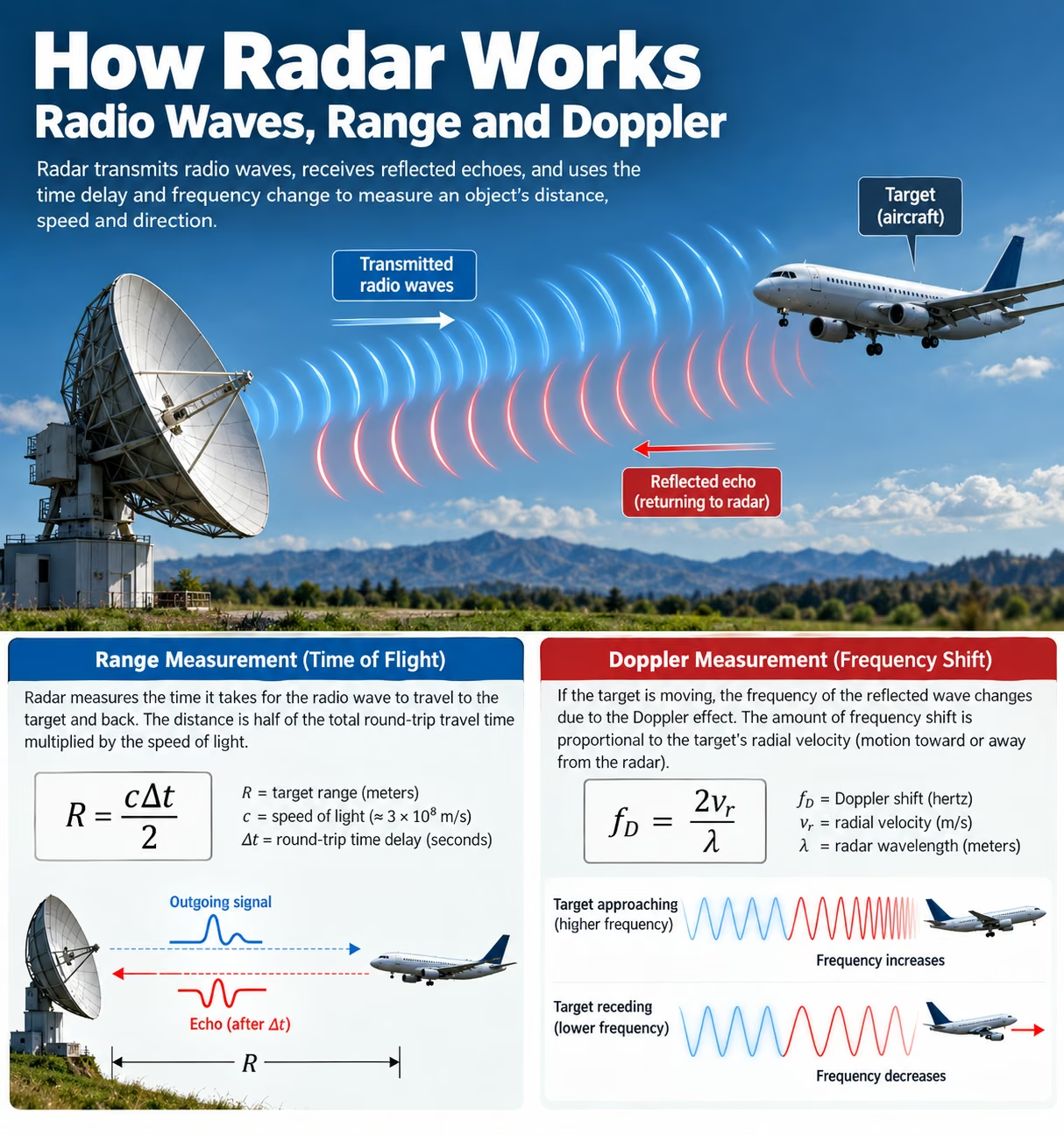
A moving object changes the phase history of the electromagnetic signal received by a radar. If a target moves toward the radar, the round-trip propagation path becomes shorter over time. If it moves away, the path becomes longer.
For a stationary monostatic radar and a conventional nonrelativistic approximation, approaching motion produces a higher received frequency and receding motion produces a lower received frequency.
The measurable shift depends only on the line-of-sight component of relative motion.
An object moving directly sideways relative to the radar can have zero instantaneous radial velocity even though its actual speed is substantial.
Coherent radar systems retain a stable phase reference, allowing very small changes in echo phase across measurements to reveal motion.
6.3. What Is the Radar Doppler Shift Equation?
For monostatic radar, where a target’s radial speed is much smaller than the speed of light, the Doppler relationship is:
For this equation, define vr as positive when the target is approaching the radar and negative when it is receding. Thus, fD=freceived-ftransmitted is positive for approaching motion.
Where:
- fD = Doppler frequency shift in hertz
- vr = signed radial velocity in meters per second
- λ = transmitted wavelength in meters
The factor of two arises because the radar signal travels to the moving target and then returns.
Different fields and processing systems may adopt the opposite sign convention. Meteorological radar products commonly use positive velocity for motion away from the radar. The physical relationship remains the same when signs are applied consistently. [3]
6.4. Example: What Doppler Shift Does a Moving Vehicle Produce?
Suppose a 24 GHz radar observes a vehicle moving directly toward it at 20 meters per second, equivalent to 72 kilometers per hour.
First, calculate the transmitted wavelength:
Next, calculate the Doppler shift magnitude:
The echo has a Doppler frequency shift of approximately 3.2 kHz.
Although this is tiny compared with the 24 GHz carrier frequency, coherent radar receivers can measure such differences after frequency conversion and signal processing.
This calculation assumes motion directly along the radar’s line of sight.
6.5. What Is the Difference Between Radial Velocity and Actual Speed?
Radial velocity is the component of an object’s velocity along the line connecting the radar and the object. Actual speed describes the magnitude of the object’s complete velocity vector.
If an object moves at speed v and the angle between its motion and the line toward the radar is θ, its radial-speed magnitude is:
When the object moves directly toward or away from the radar, the measured radial-speed magnitude equals its actual speed.
When it moves perpendicular to the radar beam, its radial velocity is zero at that instant.
This difference produces the well-known cosine effect in traffic radar. A radar positioned at an angle to a vehicle’s travel direction normally measures a smaller radial-speed magnitude than the vehicle’s actual speed, unless additional geometry correction is applied.
7. How Does Doppler Radar Measure Speed?
Doppler radar measures motion by observing frequency or phase changes in reflected electromagnetic signals. The specific method depends on whether the radar transmits continuously or in pulses. Some radars estimate speed without measuring absolute distance, while others combine range measurement with coherent Doppler processing. Signal mixing, Fourier analysis, and moving-target filters make it possible to identify moving objects even when stationary buildings, terrain, and other reflectors generate stronger echoes.
7.1. What Is Continuous-Wave Doppler Radar?
Continuous-wave (CW) Doppler radar transmits a radio-frequency signal continuously instead of sending isolated pulses. A conventional unmodulated CW radar compares the received signal with a reference derived from its transmitted carrier.
If a target moves relative to the radar, the received signal contains a Doppler shift proportional to its radial velocity.
This makes CW Doppler radar suitable for speed measurement and motion detection.
However, a conventional unmodulated CW radar cannot independently determine a target’s absolute distance because its steady transmitted waveform lacks an identifiable timing reference for round-trip delay.
More sophisticated continuous-wave systems overcome this limitation by introducing frequency, phase, or other modulation.
7.2. How Does a Radar Detect Frequency Differences?
A radar receiver can detect small frequency differences using a process called mixing. A nonlinear mixer combines two signals and produces components related to their sum and difference frequencies.
For example, when a radar transmits at 24 GHz and receives an echo shifted by 3.2 kHz, suitable mixing can produce a low-frequency component corresponding to that difference.
This lower-frequency output is easier to digitize and analyze than the original microwave carrier.
The resulting signal is often called a beat signal in radar receiver architecture.
A single real-valued mixer output generally does not preserve enough information to distinguish positive and negative Doppler frequencies reliably. In-phase and quadrature demodulation solves this by producing a complex signal whose phase rotation reveals Doppler direction.
7.3. What Is Pulse-Doppler Radar?
Pulse-Doppler radar combines pulsed ranging with coherent velocity measurement. It transmits a sequence of pulses and measures the returning echoes in successive pulse repetition intervals.
Echo delay provides range information, while changes in echo phase across pulses provide radial velocity.
For a moving target, the signal phase changes predictably as the target’s distance changes. Doppler processing estimates the frequency associated with this progression.
A pulse-Doppler radar can therefore estimate both range and radial velocity for the same target.
Coherent processing also helps separate moving targets from stationary clutter. However, pulse repetition frequency creates important constraints on range ambiguity and unambiguous Doppler velocity.
7.4. What Are Doppler Filters?
Doppler filters separate radar returns according to their Doppler-frequency content. Since different radial velocities produce different Doppler shifts, filtering can help distinguish targets with different motion characteristics.
A common processing technique collects complex signal samples across multiple radar pulses and applies an FFT along the pulse sequence.
The resulting Doppler spectrum contains frequency bins associated with different radial velocities.
By examining these bins, a radar can separate stationary or slow-moving clutter from returns representing faster movement.
The effectiveness of Doppler filtering depends on the coherent observation interval, pulse repetition strategy, clutter properties, signal-to-noise ratio, and target dynamics.
7.5. What Are Moving Target Indication and Blind Speeds?
Moving Target Indication (MTI) is a radar processing technique designed to suppress echoes from stationary or slowly moving reflectors while preserving returns from moving targets.
Traditional MTI filters compare signals from successive pulses. Stationary echoes tend to remain similar, allowing cancellation, while moving-target echoes exhibit phase changes.
However, certain target Doppler frequencies can fall at or near filter-response nulls. A moving target at one of these frequencies may be strongly attenuated.
These conditions are called blind speeds.
For a simple two-pulse canceller, nulls repeat at integer multiples of the PRF in Doppler frequency. The corresponding radial-speed magnitudes are related to nλ PRF/2, where n is an integer.
Modern radar systems use more advanced filter banks, multiple PRFs, and other techniques to reduce such limitations. [1][6]
8. What Is FMCW Radar and How Does It Measure Range and Velocity?
Frequency-modulated continuous-wave (FMCW) radar is widely used in modern automotive, industrial, and short-range sensing applications. Unlike a conventional unmodulated CW radar, FMCW changes its transmitted frequency in a controlled pattern. The returning echo represents an earlier version of the transmitted waveform, so the frequency difference contains range information. By observing multiple frequency sweeps and their phase changes, the radar can also estimate radial velocity and construct a range-Doppler representation of surrounding objects.
8.1. What Does FMCW Stand For?
FMCW stands for Frequency-Modulated Continuous Wave. It describes radar systems that transmit signals whose instantaneous frequency varies according to a prescribed modulation pattern.
Instead of relying on short, separated timing pulses, FMCW radar measures the relationship between the current transmitted waveform and a delayed returned signal.
A conventional FMCW radar uses repeated frequency sweeps called chirps.
These systems are particularly common in compact millimeter-wave sensors because modern integrated circuits can generate, receive, and process high-frequency chirps efficiently.
FMCW radar supports range and velocity estimation, but its practical capabilities depend on modulation design, receiver bandwidth, sampling, and signal processing.
8.2. How Does a Chirp Signal Work?
A chirp is a waveform whose instantaneous frequency changes over time. A linear up-chirp increases in frequency at an approximately constant rate, while a down-chirp decreases in frequency.
The slope of a linear chirp is:
Where B is the swept bandwidth and T is the sweep duration.
A target reflects a delayed version of the chirp. Since the transmitted frequency is changing, the earlier received waveform and current transmitted waveform have different instantaneous frequencies.
Their difference provides information about round-trip propagation time.
The diagram is conceptual and omits receiver timing, target motion, and other practical complications.
8.3. How Does Beat Frequency Reveal Target Distance?
For a stationary target and a linear chirp, the magnitude of the ideal beat frequency is:
Where:
- fb = beat-frequency magnitude
- S = chirp slope in Hz/s
- R = target range
- c = propagation speed
Rearranging:
Suppose a radar uses a chirp slope of 20×1012 Hz/s and observes a beat frequency of 2 MHz from a stationary target.
The target is approximately 15 meters away.
This simple calculation assumes an ideal linear chirp, a stationary target, and a beat frequency determined by delay rather than Doppler. For moving targets, the interpretation requires additional processing.
8.4. How Does FMCW Radar Separate Range and Velocity?
When a target moves, its returned chirp contains both delay-related information and a Doppler contribution. A single up-chirp beat-frequency measurement can therefore contain coupled range and velocity effects.
Modern FMCW radars commonly transmit many chirps in a sequence or frame.
Samples collected within each chirp are processed to identify range-related frequency components. The phase progression at a given range across successive chirps is then analyzed to estimate Doppler frequency.
This two-dimensional processing separates many targets according to both distance and radial motion.
Alternative waveform designs use combinations of up-chirps, down-chirps, or more complex modulation patterns.
Nevertheless, range-Doppler coupling, aliasing, interference, and moving-target effects can bias estimates unless handled appropriately. [7]
8.5. What Is a Range-Doppler Map?
A range-Doppler map is a two-dimensional representation of radar returns organized by distance and radial velocity. Each location in the map represents a combination of a range bin and a Doppler bin.
The map is commonly produced through two stages of spectral processing:
- A range FFT extracts range-related frequency information.
- A Doppler FFT evaluates phase progression across pulses or chirps.
Bright or high-intensity regions represent stronger signal energy at particular range-velocity combinations.
Range-Doppler maps help radar systems distinguish targets at similar distances but different velocities. However, a strong peak is not automatically a valid target. Clutter suppression, thresholding, CFAR detection, angular estimation, and tracking may be needed before a return becomes a confirmed object. [7][8]
9. What Limits Radar’s Ability to Measure Range and Speed Accurately?
Radar measurements are affected by both physical limitations and engineering trade-offs. A radar can receive a detectable echo yet assign it to an incorrect distance or velocity if the waveform’s ambiguity limits are exceeded. In addition, background reflections, receiver noise, interference, and multipath propagation can obscure useful returns. Reliable radar design therefore requires appropriate pulse timing, waveform bandwidth, coherent observation intervals, calibration, and processing methods that reduce false detections without discarding important targets.
9.1. What Is Range Ambiguity?
Range ambiguity occurs when a radar cannot determine which transmitted pulse produced a particular received echo. This commonly happens when an echo from a distant target arrives after a later pulse has already been transmitted.
Consider a radar transmitting 1,000 pulses per second. Its pulse repetition interval is 1 millisecond, corresponding to a nominal unambiguous range of 150 kilometers.
An echo returning after more than one pulse repetition interval can appear to belong to the wrong pulse and be assigned a shorter apparent range.
This phenomenon is also called range folding.
Radar engineers address range ambiguity using multiple PRFs, pulse coding, staggered timing, and signal association techniques. [5]
9.2. What Is Doppler Ambiguity?
Doppler ambiguity occurs when the radar’s sampling strategy cannot uniquely distinguish the Doppler frequencies produced by different radial velocities.
For a conventional uniformly sampled pulse-Doppler radar, Doppler measurements are sampled at the pulse repetition frequency. According to the Nyquist-Shannon sampling principle, signed frequencies outside the interval from -PRF/2 to +PRF/2 can alias into that interval.
The corresponding conventional monostatic unambiguous velocity condition is:
For a radar operating at a wavelength of 0.1 meter and PRF of 1,000 Hz:
Radial velocities outside this interval can produce Doppler measurements that appear to represent different velocities.
Advanced processing can sometimes resolve these ambiguities, but a single uniformly sampled Doppler sequence does not uniquely reveal all possible velocities. [5]
9.3. Why Must Radar Designers Balance Range and Velocity Ambiguity?
In a conventional pulse-Doppler radar, pulse repetition frequency creates a fundamental design trade-off.
Reducing PRF increases the interval between pulses, allowing more time for distant echoes to return before another pulse is transmitted. This increases the nominal unambiguous range.
However, reducing PRF also lowers the Nyquist Doppler frequency and the corresponding unambiguous radial-velocity interval.
Increasing PRF has the opposite effect.
| PRF, at 10 GHz | Nominal unambiguous range | Signed velocity limit |
|---|---|---|
| 1,000 Hz | 150 km | ±7.5 m/s |
| 2,000 Hz | 75 km | ±15 m/s |
| 5,000 Hz | 30 km | ±37.5 m/s |
These values use a 3 cm wavelength and idealized conventional pulse-Doppler assumptions.
Designers use staggered PRFs, multiple waveform modes, and ambiguity-resolution algorithms to manage this range-velocity trade-off. [5]
9.4. How Do Clutter and Multipath Affect Radar?
Clutter refers to radar echoes from unwanted environmental scatterers. Common examples include terrain, buildings, vegetation, sea waves, rain, and other objects not relevant to a particular measurement task.
Ground clutter can be especially strong because large stationary surfaces may reflect much more energy than small moving targets.
Multipath propagation occurs when signals travel along several paths, often after reflecting from the ground or nearby structures. These paths can produce additional delayed signals, interference between returns, or apparent targets at incorrect positions.
Doppler filtering can suppress some stationary clutter, while spatial filtering and adaptive processing can reduce selected interference sources.
However, clutter rejection is a trade-off. A slowly moving or stationary target may also be suppressed by processing designed to remove low-Doppler returns.
9.5. How Does Noise Influence Radar Detection?
Every practical radar receiver encounters noise. Thermal noise originates from random electrical fluctuations and is influenced by temperature, receiver bandwidth, and noise figure.
A weak echo must compete with noise and other unwanted signals. Detection algorithms therefore compare measured signal characteristics with criteria intended to distinguish targets from random fluctuations.
An important metric is the signal-to-noise ratio:
Higher SNR generally makes target detection and parameter estimation more reliable.
However, the performance of a radar detector is also described by its probability of detection and probability of false alarm.
Lowering the detection threshold may reveal weaker objects, but it can also increase false alarms. Raising the threshold may suppress false alarms while causing weak targets to be missed.
9.6. What Is Constant False Alarm Rate Processing?
Constant False Alarm Rate (CFAR) processing is an adaptive radar detection technique that adjusts detection thresholds according to estimates of local noise or clutter conditions.
Instead of applying a single fixed threshold across an entire radar observation, a CFAR detector examines nearby reference cells to estimate the background level around a candidate detection.
For example, a radar analyzing a range-Doppler map may compare a strong peak with the surrounding cells. If the peak sufficiently exceeds its estimated background, it becomes a candidate detection.
Different CFAR algorithms use different background-estimation strategies, including cell averaging, greatest-of, smallest-of, and ordered-statistic methods.
CFAR is designed to maintain a specified false alarm behavior under particular statistical assumptions. It cannot guarantee a perfectly constant false alarm rate in every environment, especially around clutter boundaries or multiple closely spaced targets. [8]
10. How Does Radar Determine an Object’s Direction and Track Its Motion?
Distance and Doppler velocity do not fully describe an object’s location or trajectory. Radar systems often need angular measurements to determine where a target is positioned and repeated observations to establish where it is going. Modern systems combine antenna beam patterns, phased arrays, direction-of-arrival estimation, detection association, and statistical tracking algorithms. These methods transform individual echoes into more stable position and motion estimates while accounting for measurement uncertainty and occasional missed detections.
10.1. How Does Radar Measure Azimuth and Elevation?
Azimuth is the horizontal bearing of a target relative to a reference direction, usually north. Elevation is the vertical angle between the radar’s horizontal reference plane and the direction toward the target.
A mechanically scanned radar can estimate angular direction using the antenna’s pointing angle when an echo is detected.
Electronically scanned arrays can estimate direction using the phase or time relationships between signals received at multiple antenna elements.
Angular resolution depends on antenna aperture, wavelength, processing, and signal conditions. For an ordinary filled aperture, beamwidth scales approximately with wavelength divided by aperture dimension.
A two-dimensional surveillance radar may provide range and azimuth, while a three-dimensional system can additionally estimate elevation.
10.2. What Is the Difference Between Monostatic and Bistatic Radar?
A monostatic radar places its transmitter and receiver at essentially the same location, often sharing an antenna through appropriate transmit-receive switching or isolation circuitry.
A bistatic radar uses spatially separated transmitter and receiver locations. This changes the geometry of the electromagnetic signal path.
For monostatic radar, round-trip distance is approximately twice the radar-to-target range. For bistatic radar, propagation distance is the sum of the transmitter-to-target and target-to-receiver distances.
The signal’s delay and Doppler shift therefore depend on the bistatic geometry.
Bistatic radar can offer different observation perspectives and scattering characteristics, but it also creates additional challenges involving synchronization, localization, and waveform interpretation.
10.3. How Does Target Tracking Work?
Radar target tracking connects detections across successive measurements to estimate an object’s movement through time.
For example, a radar may detect an aircraft at one location, then observe it again several seconds later. A tracking algorithm evaluates whether the detections likely came from the same aircraft and estimates its position and motion.
This process is called data association.
The resulting target track may contain estimated position, velocity, acceleration, identification information, and uncertainty.
Tracking algorithms must account for measurement errors, missed detections, new objects entering the observed region, and situations where several targets move close together.
By maintaining continuity between measurements, tracking can provide a more useful representation of movement than isolated radar detections.
10.4. How Does a Kalman Filter Improve Radar Tracking?
A Kalman filter is a mathematical estimation method used to combine predictions with noisy measurements. The classical Kalman filter, associated with Rudolf E. Kalman, provides optimal linear estimation under specified assumptions, including appropriate noise models.
Radar tracking commonly involves two stages.
During the prediction stage, a motion model estimates where a tracked object should be at the next measurement time.
During the update stage, the algorithm adjusts that prediction using the new radar observation and its estimated uncertainty.
The filter also maintains a covariance matrix that represents uncertainty in estimated states.
For nonlinear radar measurements, systems may use extended Kalman filters, unscented Kalman filters, or other estimation approaches.
Radar measurements can also be combined with information from cameras, lidar, GNSS, or inertial sensors through sensor fusion.
10.5. Can Radar Identify What Type of Object It Detects?
Radar can contribute to target classification by examining measured characteristics such as range, radial velocity, radar cross section, movement patterns, polarization response, and signal fluctuations.
One useful feature is the micro-Doppler signature, which describes Doppler components associated with motion within a target.
For example, a drone’s rotating propellers can produce additional Doppler-frequency components beyond those associated with the motion of the drone’s main body.
Human limb movements may similarly create characteristic variations in returned signals.
These signatures can help distinguish object categories, especially when combined with tracking or machine-learning methods.
Nevertheless, radar classification is probabilistic. Different objects can produce similar signatures, and classification performance depends strongly on viewing geometry, sensor resolution, signal quality, and training or modeling assumptions.
11. What Are the Major Types of Radar and Their Applications?
Radar is used wherever distance, movement, direction, or electromagnetic scattering information helps solve a practical problem. Weather radar observes precipitation and atmospheric motion, traffic radar estimates vehicle speed, and automotive radar supports collision avoidance. Aviation and marine systems monitor objects across large operational areas, while specialized radars investigate underground structures or produce images of Earth’s surface. Although these systems share electromagnetic principles, their waveforms, antennas, frequencies, and processing methods are adapted to different environments and measurement requirements.
11.1. How Does Weather Radar Detect Rain and Storm Movement?
Weather radar transmits radio waves into the atmosphere and measures energy scattered back from hydrometeors such as raindrops, snowflakes, and hailstones.
A primary measurement is radar reflectivity, commonly displayed in dBZ, which relates to the strength of precipitation scattering within a sampled volume.
Doppler weather radar also measures the radial velocity of scatterers along the radar beam.
The United States NEXRAD network uses WSR-88D Doppler weather radars to support precipitation monitoring, severe-weather analysis, and forecasting.
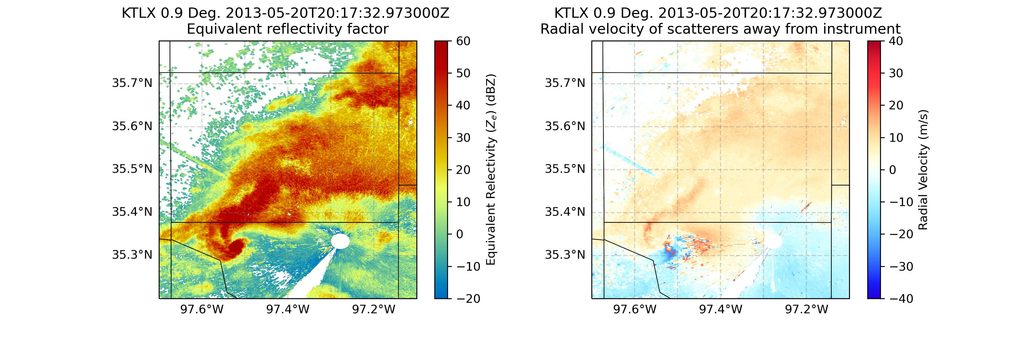
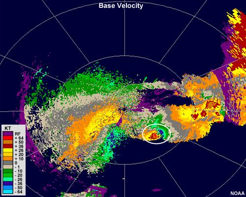
The Doppler velocity field can reveal patterns associated with atmospheric circulation, wind shear, and storm rotation. However, a single radar does not directly measure the complete three-dimensional wind vector.
Weather radar observations also depend on beam elevation, range, attenuation, precipitation properties, and ground clutter. [2][3][9]
11.2. How Does Traffic Speed Radar Measure Vehicle Speed?
Traffic speed radar uses the Doppler effect to estimate how quickly a vehicle is moving along the radar’s line of sight.
Many traditional speed-measuring radar devices operate using continuous-wave Doppler principles, comparing the transmitted radio frequency with the returned signal.
The measured Doppler shift is converted to radial speed using the radar’s wavelength.
When the radar beam is not aligned with the vehicle’s direction of travel, the cosine relationship can cause the radial-speed reading to be smaller than the actual vehicle speed.
Practical accuracy also depends on correct target selection, device calibration, interference management, reflections, and operating procedures.
A radar speed reading should therefore be interpreted as a measurement produced under specific geometric and instrumental conditions.
11.3. How Does Automotive Radar Support Driver Assistance?
Automotive radar helps vehicles monitor surrounding objects and estimate their relative distance, radial velocity, and direction.
Modern systems frequently operate near 77 GHz using FMCW techniques and multiple antenna channels.
These sensors support functions such as adaptive cruise control, forward collision warning, blind-spot monitoring, and emergency braking systems.
Multiple receiving antennas can provide angular information, while tracking algorithms associate detections with vehicles, pedestrians, and other objects.
Automotive radar is useful in darkness and some adverse visibility conditions, but it can still encounter multipath, interference, poor target geometry, or weak reflections.
Driver-assistance systems therefore often combine radar with cameras and other sensing technologies to improve environmental understanding.
11.4. How Does Marine Radar Help Ships Navigate?
Marine radar assists navigation by detecting vessels, coastlines, navigation marks, and other objects that reflect radio waves.
Many marine systems operate in X-band or S-band, with the choice affecting antenna characteristics, target discrimination, and performance in precipitation.
A ship’s radar measures target range and bearing, allowing navigators to estimate relative positions.
Automatic Radar Plotting Aid (ARPA) systems process successive observations to estimate target movement, closest point of approach, and time to closest point of approach.
These estimates support collision avoidance but do not replace proper lookout and navigational judgment.
Sea clutter, rain clutter, antenna height, target radar cross section, and vessel movement can affect performance, especially for small objects close to the sea surface.
11.5. How Does Air Traffic Control Radar Monitor Aircraft?
Air traffic control radar supports aircraft surveillance by providing information about aircraft locations and movement within monitored airspace.
Primary surveillance radar (PSR) detects reflected radio signals without requiring an aircraft to transmit a cooperative reply.
Secondary surveillance radar (SSR) uses interrogations and aircraft transponder responses to obtain information such as identification and reported altitude.
The FAA’s ASR-11 airport surveillance radar integrates primary and secondary radar capabilities for terminal air traffic surveillance.
Primary radar can measure range and azimuth from reflected energy, while secondary radar can supplement surveillance with cooperative aircraft information.
Modern air traffic surveillance can also use ADS-B and other systems, which have distinct operating principles.
Radar remains an important component of aviation surveillance, particularly where independent target detection or supplementary coverage is required. [10]
11.6. How Does Radar Measure Aircraft Height Above the Ground?
A radar altimeter measures an aircraft’s height above the reflecting surface beneath it, commonly referred to as height above ground level in this context.
Unlike a barometric altimeter, which estimates altitude relative to a pressure reference, a radar altimeter uses radio waves to measure the distance toward terrain or another reflecting surface below the aircraft.
Many radio altimeters use FMCW ranging principles.
The aircraft transmits a downward-directed signal and analyzes its return to estimate clearance.
This measurement is important during low-altitude operations, landing, and certain automatic flight-control functions.
A radar altimeter does not directly measure altitude above mean sea level, and its reading can depend on terrain, surface reflectivity, attitude, and system design.
11.7. How Does Ground-Penetrating Radar Detect Underground Objects?
Ground-penetrating radar (GPR) transmits electromagnetic waves into the ground and measures reflections from boundaries between materials with different electromagnetic properties.
Unlike conventional radar operating predominantly through air, GPR signals propagate through soil, rock, concrete, or other materials.
Their propagation speed depends strongly on dielectric permittivity, while attenuation is influenced by electrical conductivity and other material properties.
A reflection may occur where the wave encounters a buried pipe, rock boundary, void, or change in soil composition.
GPR is used in archaeology, utility location, pavement assessment, geological investigation, and civil engineering.
Penetration depth varies significantly with ground conditions. Electrically conductive, clay-rich, or saline materials can strongly attenuate signals and limit useful detection depth. [11]
11.8. What Is Synthetic Aperture Radar?
Synthetic Aperture Radar (SAR) is an imaging radar technique that uses coherent measurements collected as a radar platform moves along a path.
Instead of relying exclusively on the physical antenna length for along-track resolution, SAR processing combines measurements taken at multiple positions to synthesize the effect of a much larger antenna aperture.
This allows aircraft and satellites to produce detailed radar images of Earth’s surface.
SAR can acquire imagery during darkness and through many cloud conditions, making it especially useful for environmental monitoring.
The European Space Agency’s Sentinel-1 mission uses C-band SAR at approximately 5.405 GHz. Its applications include monitoring floods, sea ice, land movement, maritime conditions, and environmental change.
SAR interferometry can also compare the phase of compatible acquisitions to estimate surface deformation under suitable conditions. [12]
12. How Are Radar Systems Tested, Calibrated, and Evaluated?
Radar performance must be measured under controlled and realistic operating conditions. A theoretically capable radar may still produce inaccurate measurements if its timing, antenna pointing, frequency reference, gain, or receiver characteristics are not properly calibrated. Engineering evaluation therefore includes both laboratory measurements and field trials. Tests examine whether the system can detect expected targets, estimate their parameters accurately, maintain acceptable false alarm rates, and continue performing reliably as environmental and operating conditions change.
12.1. What Is Radar Calibration?
Radar calibration is the process of checking and adjusting radar measurements against known references.
Depending on the system, calibration may address transmitted power, receiver gain, timing accuracy, frequency stability, antenna alignment, phase relationships, polarization, and signal-processing behavior.
Engineers may use reference reflectors, calibrated signal generators, known target positions, or specialized test equipment.
For example, a radar designed to measure distance can be tested against a target positioned at a known range. Any systematic difference between measured and reference distance can indicate timing or processing errors.
Calibration should be distinguished from performance validation. Calibration establishes measurement consistency, while validation examines whether the complete system meets its operational requirements.
12.2. Which Metrics Describe Radar Performance?
Radar performance cannot be represented by a single specification. Maximum detection range describes coverage under defined assumptions, while range resolution determines whether closely separated targets can be distinguished. Velocity resolution, angular resolution, sensitivity, and detection reliability describe other aspects of the system.
| Performance metric | What it describes |
|---|---|
| Maximum detection range | Greatest distance at which specified detection criteria are met |
| Range resolution | Ability to separate targets at nearby distances |
| Range accuracy | Agreement between estimated and actual distance |
| Angular resolution | Ability to distinguish targets by direction |
| Velocity resolution | Ability to separate nearby Doppler velocities |
| Unambiguous range | Distance interval before conventional range folding |
| Unambiguous velocity | Velocity interval before conventional Doppler aliasing |
| SNR | Signal strength relative to noise |
| Probability of detection | Likelihood of detecting a target under specified conditions |
| False alarm probability | Likelihood of reporting a detection without a target |
| Receiver sensitivity | Weak-signal detection capability under defined conditions |
Each metric depends on waveform design, integration, processing, target characteristics, and operating environment. Meaningful comparisons require consistent measurement conditions.
12.3. How Do Engineers Evaluate Detection Accuracy?
Engineers evaluate radar accuracy by comparing its measurements with reliable reference information obtained through controlled target arrangements, calibrated equipment, or independent measurement systems.
Laboratory testing may use signal simulators, known RF inputs, controlled propagation environments, and reference reflectors.
Field testing assesses performance in realistic conditions involving environmental clutter, interference, weather, and moving targets.
Measurements commonly include systematic error, statistical variation, detection probability, missed detections, and false alarms.
For example, a radar may repeatedly measure a target slightly farther away than its actual location. That pattern suggests a systematic range bias.
A different radar may produce estimates distributed around the correct range but with substantial variation, indicating lower precision.
Engineers also assess tracking continuity, latency, target separation, and performance at different distances and viewing angles.
13. Radar Formulas and Worked Examples
Radar engineering uses a relatively small set of fundamental equations to calculate distance, wavelength, Doppler velocity, range resolution, received power, and ambiguity limits. These equations are useful for understanding radar systems, but their assumptions must be respected. Most introductory calculations treat electromagnetic propagation through air as occurring at 3×10⁸ meters per second. Real radar performance also depends on waveform characteristics, measurement uncertainty, target geometry, propagation losses, and signal processing.
13.1. How Do You Calculate Distance From Radar Echo Delay?
To calculate target distance from echo delay, multiply the measured round-trip travel time by the propagation speed and divide by two. The factor of two accounts for the outward and returning signal paths.
For an echo delay of 50 microseconds:
This calculation is appropriate for an idealized monostatic system.
For a conventional radar operating through air, every additional microsecond of round-trip delay corresponds to approximately 150 meters of additional range.
{@body const [delay,setDelay]=DIL.useState(20)}
13.2. How Do You Calculate Radar Wavelength From Frequency?
Radar wavelength is calculated by dividing the propagation speed by the transmitted frequency.
For a 10 GHz radar:
The wavelength is 3 centimeters.
| Radar frequency | Approximate wavelength |
|---|---|
| 3 GHz | 10 cm |
| 10 GHz | 3 cm |
| 24 GHz | 1.25 cm |
| 77 GHz | 3.90 mm |
Shorter wavelengths produce larger Doppler frequency shifts for the same radial velocity. They can also support narrower antenna beams for the same physical aperture.
However, wavelength alone does not determine range resolution, detection capability, or overall performance.
13.3. How Do You Calculate Target Speed From Doppler Shift?
The magnitude of radial velocity can be calculated from the Doppler frequency shift and radar wavelength.
Suppose a 10 GHz radar measures a Doppler shift magnitude of 2,000 Hz.
Its wavelength is:
The radial-speed magnitude is:
Converting to kilometers per hour:
The measured radial-speed magnitude is 108 km/h.
This equals actual object speed only if the motion is directly along the radar’s line of sight. Otherwise, the measurement represents a component of the full velocity.
13.4. How Do You Calculate Range Resolution From Bandwidth?
For suitable radar waveforms, the commonly used range-resolution approximation is:
Here, B is the effective signal bandwidth.
Increasing the bandwidth decreases the nominal distance separation required to distinguish two targets.
| Waveform bandwidth | Nominal range resolution |
|---|---|
| 150 MHz | 1.00 m |
| 500 MHz | 0.30 m |
| 1 GHz | 0.15 m |
A 1 GHz bandwidth produces a nominal range resolution of approximately 15 centimeters.
This does not mean every object’s distance will have exactly 15 centimeters of measurement error. Range resolution and range accuracy are separate performance characteristics, and practical results depend on processing, SNR, and waveform design.
13.5. How Do You Calculate the Unambiguous Range of Pulse Radar?
For a conventional pulse radar with a constant pulse repetition frequency, nominal unambiguous range is:
Consider a radar operating at a PRF of 2,000 Hz:
At a lower PRF of 1,000 Hz, this increases to 150 km.
At 5,000 Hz, it decreases to 30 km.
These values describe pulse-timing ambiguity, not the maximum target distance at which sufficient received power is available. A radar may detect a return beyond its nominal unambiguous range but require additional processing to identify the correct distance.
13.6. How Do You Calculate Received Radar Power?
The simplified monostatic radar equation estimates received power from transmitted power, antenna gain, wavelength, radar cross section, target distance, and losses.
Consider the following idealized radar:
- Transmitted power: 1,000 W
- Antenna gain: 1,000, or 30 dBi
- Wavelength: 0.03 m
- Target radar cross section: 1 m²
- Target range: 10,000 m
- Loss factor: 1
Substituting:
This is approximately −103.4 dBm.
The calculation demonstrates how small radar echoes can become even when a relatively powerful transmitter and high-gain antenna are used.
Holding the equation’s other quantities constant, doubling target distance reduces received power by a factor of 16. Doubling linear antenna gain on both transmit and receive increases received power fourfold.
Actual detection performance must additionally account for noise, processing gains and losses, propagation, and target fluctuations.
13.7. How Do You Calculate FMCW Range From Beat Frequency?
For a stationary target observed using an ideal linear FMCW chirp, range is related to beat-frequency magnitude and chirp slope.
Suppose the radar’s chirp slope is 30×1012 Hz/s and the measured beat frequency is 4 MHz.
The estimated target distance is 20 meters.
For moving targets, the beat signal can include Doppler contributions. Real FMCW systems commonly use multiple chirps and coherent processing to estimate range and velocity separately. [7]
14. Frequently Asked Questions About Radar, Radio Waves, and Doppler
Radar terminology can be confusing because words such as range, resolution, velocity, frequency, and detection describe different properties of the sensing process. Some radar systems detect stationary targets, while others are specifically optimized to recognize movement. Likewise, particular frequencies provide advantages in some environments but disadvantages in others. The following questions clarify the most common misconceptions about radar operation, including its ability to work in darkness, measure speed without distance, and distinguish multiple objects.
14.1. Does Radar Use Radio Waves or Microwaves?
Radar uses radio-frequency electromagnetic waves. Many radar systems operate at microwave frequencies, which are a portion of the broader radio spectrum. Therefore, describing radar as using microwaves and describing it as using radio waves are both correct for microwave radar systems.
Microwave frequencies are practical because they can be generated electronically, directed using antennas, and used to investigate objects and surfaces.
Not all radars operate at the same frequency. Some use longer radio wavelengths for surveillance and specialized remote sensing, while automotive sensors often use millimeter waves.
The chosen frequency influences antenna size, propagation characteristics, scattering behavior, and available waveform bandwidth.
14.2. Why Does Radar Divide the Travel Time by Two?
A conventional monostatic radar measures the total time required for a signal to travel from the radar to an object and return. This is a round-trip measurement, so the wave covers approximately twice the one-way distance.
If the radar simply multiplied the complete delay by the propagation speed without dividing by two, it would calculate the total path length rather than the actual radar-to-target range.
For example, a round-trip delay of 10 microseconds represents approximately 3,000 meters of propagation. The object is only about 1,500 meters away.
This correction is built into the fundamental range equation.
14.3. Can Radar Detect an Object That Is Not Moving?
Yes. Radar does not require a target to move before it can produce a measurable return. A stationary building, parked vehicle, terrain feature, or fixed reflector can scatter transmitted radio waves back toward the receiver.
Conventional pulse radar can detect stationary objects by measuring the arrival time and strength of their echoes.
However, some radar systems employ moving-target filters designed to suppress echoes with zero or low Doppler frequency.
In those systems, a stationary object may be intentionally removed from a particular processed output.
Therefore, whether a stationary object appears depends on the radar waveform and processing configuration, not simply on whether the object reflects radio waves.
14.4. Can Radar Measure Both Distance and Speed at the Same Time?
Yes. Pulse-Doppler and FMCW radars can estimate range and radial velocity from the same target using appropriately designed waveforms and coherent signal processing.
Pulse-Doppler radar commonly derives distance from echo delay and velocity from phase progression across repeated pulses.
FMCW radar uses frequency modulation to obtain range information and often examines phase changes across successive chirps to estimate radial velocity.
By comparison, a conventional unmodulated continuous-wave Doppler radar can measure radial speed but does not independently provide absolute range.
The ability to measure multiple parameters depends on the waveform, antenna configuration, processing, and ambiguity limits.
14.5. Does a Higher Radar Frequency Always Provide Better Resolution?
No. Higher frequency means shorter wavelength, but radar resolution depends on several different design parameters.
Range resolution is primarily associated with effective waveform bandwidth for many common radar signals. A higher carrier frequency does not automatically provide a greater absolute bandwidth.
Angular resolution depends on the relationship between wavelength and antenna aperture, so shorter wavelengths can provide an advantage when physical antenna size is fixed.
Doppler sensitivity also increases as wavelength decreases because a given radial velocity produces a larger Doppler frequency shift.
However, higher frequencies may encounter greater atmospheric losses in certain conditions and impose different hardware constraints. Overall radar performance requires balancing these factors.
14.6. Why Can Radar Measure Speed Without Measuring Distance?
A conventional continuous-wave Doppler radar can measure radial speed because motion changes the frequency of the returned electromagnetic signal.
The radar compares the transmitted carrier with the received carrier and estimates their frequency difference. Using the transmitted wavelength, it converts this Doppler shift into radial velocity.
The calculation does not require knowledge of the target’s absolute distance.
However, a steady unmodulated carrier does not provide an identifiable timing feature from which the round-trip propagation delay can be determined uniquely.
That is why conventional unmodulated CW radar can estimate radial speed without independently determining target range.
14.7. What Happens When Radar Detects Multiple Objects?
When several objects reflect radar signals simultaneously, the receiver collects a combination of their echoes.
Radar processing attempts to distinguish those returns using differences in range, Doppler velocity, angular direction, and other signal characteristics.
For example, two vehicles at different distances may appear in separate range bins. Two vehicles at similar distances but different radial speeds may be separated using Doppler processing.
Multiple antenna channels can provide additional angular discrimination.
Detection algorithms such as CFAR identify candidate returns, and tracking algorithms associate detections across successive observations.
Targets that are too close in measurement space may be difficult to resolve, creating challenges such as merged detections or incorrect track association.
14.8. Why Does Rain Affect Some Radar Frequencies More Than Others?
Rain affects radar waves through scattering and attenuation, and these effects depend on wavelength, precipitation properties, and the geometry of propagation.
When radio wavelengths are comparable to the sizes of raindrops, scattering behavior can differ significantly from that at much longer wavelengths.
At some higher microwave and millimeter-wave frequencies, precipitation attenuation can become an important limitation, particularly over long propagation paths or in intense rain.
However, atmospheric absorption and precipitation effects are frequency-dependent rather than simply increasing uniformly with frequency.
Radar designers select operating bands to balance precipitation sensitivity, coverage, antenna requirements, and attenuation.
Weather radar intentionally uses precipitation scattering to obtain information about rainfall and storms.
14.9. Can Radar See Through Walls, Clouds, or Fog?
Radar can operate through many cloud and fog conditions because some radio wavelengths are much less affected by small atmospheric droplets than visible light.
Certain radar frequencies can also penetrate some building materials, vegetation, soil, and other media.
However, penetration is not universal. Conductive materials, thick reinforced structures, water-rich materials, and certain radar frequencies may strongly attenuate or reflect the incident energy.
Radar does not simply see through all solid objects.
Whether useful measurements can be obtained depends on wavelength, material properties, transmitted power, target geometry, signal-to-noise ratio, and processing capabilities.
Ground-penetrating radar and specialized through-material sensing systems illustrate how different radar designs exploit these characteristics.
14.10. What Is the Difference Between Radar Range and Range Resolution?
Radar range describes the measured distance from the radar to a target. Range resolution describes the ability to distinguish two targets located at slightly different distances.
For example, a radar may estimate that a vehicle is 100 meters away. That is a range measurement.
If another vehicle is located at 100.2 meters, whether the radar can distinguish the two returns depends on its range resolution and other measurement conditions.
A radar with nominal range resolution of 1 meter may struggle to separate two targets whose range difference is only 20 centimeters.
Range accuracy and range resolution are also distinct. High-SNR measurements can sometimes locate a single isolated target more precisely than the radar’s nominal two-target resolution.
14.11. What Is the Difference Between Doppler Shift and Beat Frequency?
Doppler shift is a physical change in observed frequency caused by relative motion between the radar and target.
Beat frequency is the difference-frequency component produced when signals at different frequencies are combined through mixing.
In a conventional unmodulated CW Doppler radar, the beat frequency can correspond directly to the Doppler shift magnitude.
In FMCW radar, the beat frequency also contains information associated with the delay between transmitted and received chirps.
For moving FMCW targets, the observed beat signal can include both delay-related and Doppler contributions.
Therefore, the two terms are related but not interchangeable. Their relationship depends on the transmitted waveform and receiver processing.
14.12. Why Can Doppler Radar Produce Incorrect Velocity Readings?
Doppler radar velocity estimates can be affected by measurement geometry, ambiguous sampling, environmental reflections, and target association errors.
An object moving at an angle to the radar beam produces a radial velocity smaller in magnitude than its actual speed.
Doppler aliasing can cause velocities outside the unambiguous interval to appear at incorrect values.
Ground clutter, multipath propagation, interference, and receiver noise can distort the observed signal.
In multi-target environments, a radar may also associate a Doppler measurement with the wrong object.
Reliable radar measurements depend on proper calibration, waveform selection, signal processing, target discrimination, and appropriate operating procedures.
14.13. What Limits the Distance a Radar Can Detect?
Radar detection range depends on transmitted energy, antenna gain, target radar cross section, propagation losses, receiver noise, processing gain, and the chosen detection threshold.
In a simplified monostatic point-target model, received echo power decreases approximately with the fourth power of target distance.
Atmospheric absorption and scattering can introduce additional losses, while Earth curvature, terrain, and obstacles may restrict the radar’s line of sight.
Target geometry also matters because radar cross section can change greatly with viewing angle.
Increasing transmitted power or antenna gain may improve coverage, but practical radar range must be evaluated against the probability of detection and allowable false alarm rate.
14.14. What Is the Difference Between Pulse Radar and FMCW Radar?
Pulse radar transmits discrete pulses and commonly calculates target distance from the time elapsed before an echo returns.
FMCW radar transmits a frequency-modulated waveform and estimates range using the relationship between transmitted and delayed received signals.
Pulse-Doppler systems can measure velocity using phase progression across pulses, while FMCW systems commonly use repeated chirps and coherent processing to estimate Doppler velocity.
Neither architecture is automatically better for every application.
| Feature | Pulse radar | FMCW radar |
|---|---|---|
| Waveform | Discrete pulses | Frequency sweeps |
| Range measurement | Echo delay | Beat-frequency or related processing |
| Radial velocity | Coherent Doppler processing when supported | Doppler processing across chirps |
| Typical applications | Surveillance, weather, long-range radar | Automotive, industrial sensing, short-range radar |
| Key limitations | Pulse timing and Doppler ambiguity | Range-Doppler coupling, sampling and chirp constraints |
Actual capabilities depend on specific radar implementation rather than waveform category alone.
14.15. How Does Radar Distinguish a Moving Target From the Background?
Radar can distinguish moving targets from stationary background reflectors by analyzing changes in received signal phase or Doppler frequency over time.
Stationary clutter often produces near-zero Doppler frequency for a stationary radar. Moving objects may create measurable nonzero Doppler components.
Moving Target Indication processing and Doppler filters can therefore suppress selected low-frequency clutter while preserving moving-target returns.
More advanced systems combine Doppler processing with angular filtering, waveform diversity, CFAR detection, and tracking.
However, a moving target with very low radial velocity may resemble stationary clutter, while moving vegetation, rain, waves, or other environmental objects may produce nonzero Doppler returns.
Reliable discrimination requires considering both motion and the environment.
15. Conclusion: How Radio Waves, Range, and Doppler Work Together
Radar transforms electromagnetic-wave behavior into measurements of the surrounding world. It transmits radio waves, receives reflected or scattered signals, and extracts information from their timing, amplitude, frequency, phase, and direction.
The two most important measurement principles are straightforward.
Range is derived from propagation delay or an equivalent waveform-dependent measurement. For a conventional monostatic pulsed radar, the signal travels to the target and back, giving the familiar relationship R=cΔ t/2.
Radial velocity is derived from Doppler-related frequency or phase changes. For conventional monostatic radar at nonrelativistic speeds, the Doppler shift is related to radial velocity by fD=2vr/λ, using a consistent sign convention.
Modern radar systems combine these principles with powerful antennas, precisely controlled waveforms, sensitive receivers, and digital processing.
Pulse-Doppler radar estimates distance and motion using sequences of coherent pulses. FMCW radar uses frequency sweeps and beat-signal processing to determine range, with repeated chirps supporting Doppler measurement.
Phased arrays provide electronic beam steering, matched filters improve processing of coded waveforms, CFAR algorithms help identify significant returns, and tracking systems connect individual detections into estimates of an object’s movement.
Radar still faces important physical limitations. Echoes become weaker with distance, Doppler measurements represent line-of-sight velocity, and ambiguity, clutter, atmospheric attenuation, and interference can distort results.
Understanding those limitations is as important as understanding the equations themselves.
From weather forecasting and traffic monitoring to aviation safety, automotive collision avoidance, ground investigation, and satellite Earth observation, radar demonstrates how carefully measured electromagnetic signals can reveal objects and motion that would otherwise be difficult or impossible to observe.
Sources
The following authoritative technical publications, government agency documents, and radar engineering references support the measurements, formulas, and examples discussed throughout this guide.
- MIT Lincoln Laboratory. Introduction to Radar Systems. Comprehensive radar engineering course covering propagation, range equations, antennas, receivers, clutter, detection, Doppler processing, and tracking.
- National Oceanic and Atmospheric Administration (NOAA). How Radar Works. Introduction to radio-wave transmission, radar echoes, pulse timing, and Doppler weather radar.
- NOAA. Radar Images: Velocity. Explains radial velocity, beam-relative movement, and the distinction between Doppler velocity and actual target velocity.
- MIT Lincoln Laboratory. Radar Systems Course: Waveforms, Detection, and Pulse Compression. Educational coverage of range resolution, signal processing, matched filtering, and receiver architecture.
- NOAA National Severe Storms Laboratory. A Guide for Interpreting Doppler Velocity Patterns. Technical explanation of range folding, PRF, Nyquist velocity, and Doppler ambiguity.
- MathWorks. Ground Clutter Mitigation With Moving Target Indication Radar. Explains MTI filtering, clutter suppression, blind speeds, and staggered PRFs.
- Texas Instruments. Radar Academy: FMCW Radar Terminology. Technical definitions for chirps, range FFT, Doppler FFT, range resolution, and velocity processing.
-
MathWorks. Detection, Range, Angle, and Doppler Estimation. Engineering references for detection algorithms, matched filtering, CFAR, and radar parameter estimation.
Applications and operational references - NOAA National Weather Service. Radar Images: Reflectivity. Discusses precipitation scattering, reflectivity measurements, and weather radar products.
- Federal Aviation Administration (FAA). Airport Surveillance Radar: ASR-11. Official explanation of primary and secondary air traffic surveillance radar.
- United States Geological Survey (USGS). Ground-Penetrating Radar Investigations. Technical discussion of subsurface electromagnetic propagation, dielectric properties, and ground attenuation.
- European Space Agency (ESA). Sentinel-1 Synthetic Aperture Radar Instrument. Official information about C-band synthetic aperture radar, satellite imaging, and Earth observation applications. —